Discounting approach

Calculation of the LUEC metric relies upon the discounting approach, and thus on the ‘time value of money’ concept. This notion of ‘time value of money’ captures the idea that having $1 today is “worth more” than the certainty of receiving $1 in the future (say a year). The reason is that $1 today could be deposited in a bank account, earn interest (at – say – 5% per annum), and so be worth – say - $1.05 in a year.

We may draw a similar analogy between the certainty of paying out $1 in the future (say a year) and paying out $1 today: the need to pay out $1 today is a more onerous liability than the need to pay out $1 in a year’s time, because we will lose the opportunity to invest that $1 and have something in excess of $1 in a year.

Because - as outlined above – the value of money received (or paid) depends on the time at which it is received (or paid) we must recognize that when we make decisions that involve spending and receiving different cashflows at different points in time, we are “comparing apples and oranges”. Investment decisions – including decisions regarding a choice between technologies which involve different capital expenditure profiles and/or O&M cost profiles - are of this nature. In order to compare projects and/or technologies that give rise to different cashflows at different points in time we need to put these flows on a comparable basis; this is done using the discounting approach (which gives rise – as will be shown below – to a Present Value). To reiterate: discounting is a method for comparing future $ amounts with current $ amounts. It is based on the idea that we could earn interest of r per year on current $ amounts. If we deposited $100 in the bank today, then we would get back $100 × (1+r) in 1 year – where “r “ could be 0.04 (4%), 0.05 (5%), 0.06 (6%) etc. In this context, the “Present Value” (PV) of $1 to be received in 1 year is the answer to the question: What is the $ amount that – if we multiplied it by 1 + r – would give $1? We can calculate the answer to this question using discounting. For example, if we could earn 5% per annum (p.a.) on money deposited in a bank, then the certain promise of $1 in 365 days is worth (today):

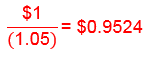
What does this mean? That you should be willing to pay $0.9524 today for the certainty of receiving $1 in 365 days. Alternatively, thinking in terms of paying out – rather than receiving - $ amounts, you should be willing to pay (up to) $0.9524 today to avoid having to pay out $1 in 365 days. The value of $0.9524 is the discounted value today of $1 in 365 days time.

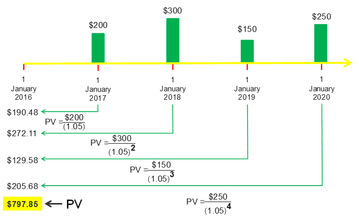
The discounting approach can be applied to any stream of cashflows (receipts or expenditures, or a mixture of both). The figure below illustrates how a cashflow profile starting in a year’s time, and subsequently extending over a four-year period can be discounted to provide a PV of $797.85 today (a 5% rate of interest is assumed).

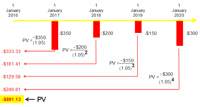
The figure below shows how the PV ($-891.13) of a stream of payments made over the same time frame can be calculated using the same discounting approach.

To arrive at the LUEC figure, this discounting approach is applied to the lifetime costs of constructing, operating and decommissioning a plant, and then ‘normalized’ by dividing by the lifetime output of that plant (also discounted) measured in kWh or MWh.