LUEC computation

The economic evaluation of competing bids will typically rely upon the Levelised Unit Electricity Cost (LUEC) metric. Computation of this ‘figure of merit’ for a given vendor’s bid involves first identifying the nature of all of the (typically ‘plant-level’) costs which will arise over the lifetime of the NPP, including the capital costs contained in the bid as well as projected fuel, Operating & Maintenance (O&M) and ‘back end’ costs (the cost of decommissioning the NPP at the end of its life, and the disposal of Spent Nuclear Fuel).

The timing profile of when these costs will arise is important, as the LUEC metric relies upon the discounting approach which – in turn – embodies the ‘time value of money’ concept: the idea that receiving a given money amount today should be valued more than the certainty of receiving an identical amount at some future date, if only because the money received today could – in principle – be invested and earn a return between today and that future date.

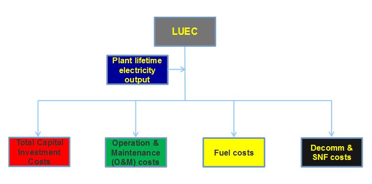
To arrive at the LUEC figure, this discounting approach is applied to the lifetime costs of constructing, operating and decommissioning a plant, and then ‘normalized’ by dividing by the lifetime output of that plant (also discounted!) measured in kWh or MWh. Schematically we represent the component inputs into a typical LUEC calculation below:

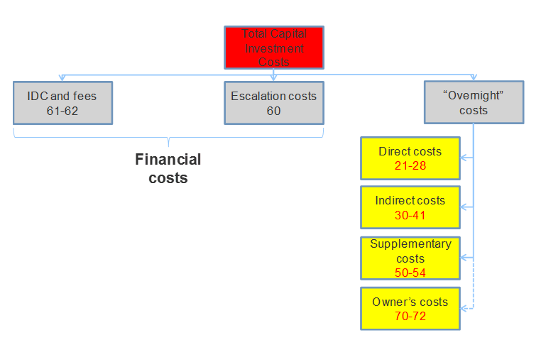
Total Capital Investment Costs (TCIC) are a key component of the LUEC for nuclear energy plant projects, typically accounting for around 2/3rds of the overall LUEC (nuclear electricity cost can be characterised as being driven by high capital costs and relatively low operating and fuel costs, unlike – for example – gas fired generation plants). TCIC can be further broken down into ‘Interest During Construction (IDC) and fees’, ‘escalation costs’ (arising from increases in input prices during the plant construction phase) and ‘overnight costs’ (the cost which would be incurred if the plant could be built ‘overnight’ at the date at which the cost estimate is being prepared). Overnight costs can be disaggregated further, as shown. Note that the numbers associated with these cost components refer to their designation in the IAEA’s ‘System of Accounts’ (see Annex I in Economic Evaluation of Bids for Nuclear Power Plants, IAEA Technical Reports Series No. 396.

Operating & Maintenance (O&M) costs include cost drivers such as wages and salaries for engineering and technical support staff and for operations, maintenance and administration staff, insurance and taxes, consumable operating materials and equipment.

Fuel costs include uranium supply, conversion, enrichment and fuel assembly fabrication, as well as components such as quality assurance and licensing assistance. It is of course possible that the project developer envisages entering into a long-term fuel supply contract with a vendor, in which case many of these drivers may not be identified separately, but rather “rolled into” an overall contract price which would be included in the LUEC.

The Decomm(issioning) and SNF (Spent Nuclear Fuel) cost component of the LUEC is identified separately in the schematic above, although their sub-components are classified within other accounts within the IAEA code of accounts. This component will include decommissioning costs, reprocessing (if this is the chosen fuel-cycle approach), final waste disposal, etc.

The final input to the LUEC calculation is the plant lifetime electricity output. Heuristically it is clear that what is of ultimate interest in comparing technologies is the cost of the electricity which they produce as measured on a (discounted) per unit of output basis. As will be shown below then, while the numerator of the LUEC metric is a cost measure, its denominator is the (discounted) time profile of station electricity generation. This will be driven – in turn – by factors such as station life (many Generation III technologies are expected to achieve station lives of up to 60 years) and the capacity factor which is expected to be achieved (capacity factors of around 90% are often employed in LUEC calculations; these may be argued to be rather optimistic – particularly in the early years of a station’s operation).

To calculate the LUEC it is necessary to identify a profile for the value of each of these inputs over the NPP project lifecycle (including the ‘back end’ of that lifecycle, i.e. the post-shutdown period during which costs will be incurred for decommissioning and disposal of waste including SNF/reprocessing waste.

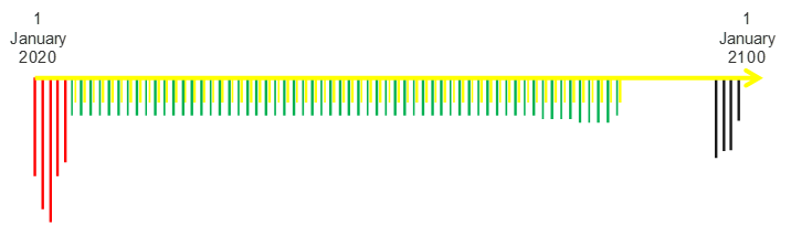
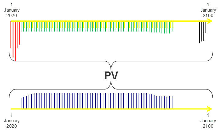
An example of such a profile is illustrated below. The hanging red bars represent a 5-year Capital Expenditure (CAPEX) profile, i.e. a distribution of the TCIC over an (assumed) 5-year construction period. The green bars represent O&M costs incurred during the station’s operating lifetime (assumed to increase then decrease at the end of the station’s life, as first more maintenance is needed on the ageing plant, and then maintenance is reduced as plant shutdown approaches); the yellow bars represent fuel costs. The black bars represent the ‘back end’ costs: decommissioning and SNF/reprocessing waste disposal. The gap between the station End of Life (EOL) and the commencement of decommissioning and waste disposal activities reflects an assumption of ‘deferred dismantling’ – i.e. that the station remains in safe storage for two or three decades before decommissioning commences. Note that the cost profile is shown undiscounted (the effect of discounting would be to increasingly ‘squeeze’ the bars shorter in successive later years, considerably reducing – for example – the bars associated with ‘back end’ costs).

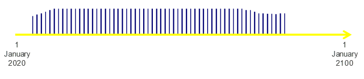
The cost profile shown above will appear in the numerator of the LUEC measure. Turning to the denominator, the LUEC relies on a projected profile for electricity output. The figure below assumes that during its operating phase the output of the plant first rises as an increasing capacity factor is driven by increasing operating experience, and remains constant throughout most of the remaining plant life, before beginning to decline as the ageing plant nears EOL. Once again it is important to note that this profile is shown undiscounted.

Given the data illustrated in the previous figures the next step in deriving the LUEC metric is discounting. It is important to note that both the cost profile and the generation output profile should be discounted (see graphic below). Broadly the rationale for discounting the flows in the denominator of the LUEC mirrors that for discounting the flows in the numerator: a unit of electricity which will (certainly) be available for use at some future date is less valuable than a unit of electricity which is available for use today. One argument in support of this rationale is that one unit of electricity which is available today could be sold, the resulting revenue invested, and the resulting revenue with interest could be used to acquire more than one unit of electricity at that future date.

A schematic of – and the results from - a typical LUEC calculation exercise are shown below (numbers are purely for illustrative purposes). As shown in the decomposition, capital costs (TCIC) are the most significant driver of the overall LUEC. The role of discounting is very apparent in the relatively insignificant contribution which ‘back end’ costs make to the overall LUEC figure. Crucially, although these costs are large they are incurred a long time in the future – and are thus heavily discounted.

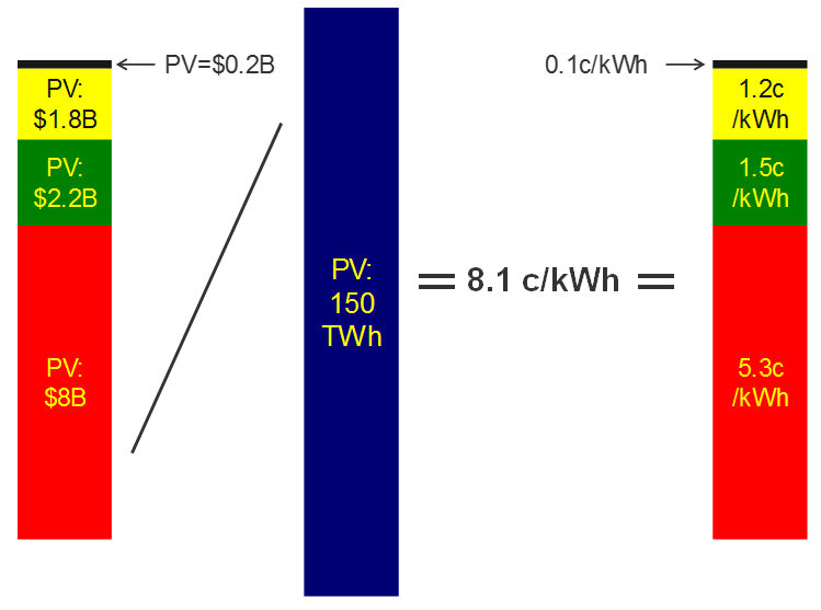
Conceptually – as shown – the use of LUEC as a metric by which to compare the economic advantages offered by different bids is relatively straightforward. In practice there may be significant challenges in using such a metric – including the choice of a discount rate.